03. Pre-Lab: Student Admissions in Keras
Mini Project: Student Admissions in Keras
So, now we're ready to use Keras with real data. We'll now build a neural network which analyzes the dataset of student admissions at UCLA that we've previously studied.
As you follow along with this lesson, you are encouraged to work in the referenced Jupyter notebooks at the end of the page. We will present a solution to you, but please try creating your own deep learning models! Much of the value in this experience will come from playing around with the code in your own way.
Workspace
To open this notebook, you have two options:
- Go to the next page in the classroom (recommended)
- Clone the repo from Github and open the notebook StudentAdmissionsKeras.ipynb in the student_admissions_keras folder. You can either download the repository with
git clone https://github.com/udacity/deep-learning.git, or download it as an archive file from this link.
Instructions
This is more of a follow-along lab. We'll show you the steps to build the network. However, at the end of the lab you'll be given the opportunity to improve the model, and try to improve on its performance. Here are the main steps in this lab.
Studying the data
The dataset has the following columns:
- Student GPA (grades)
- Score on the GRE (test)
- Class rank (1-4)
First, let's start by looking at the data. For that, we'll use the read_csv function in pandas.
import pandas as pd
data = pd.read_csv('student_data.csv')
print(data)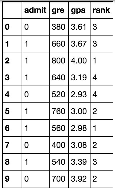
Here we can see that the first column is the label y, which corresponds to acceptance/rejection. Namely, a label of 1 means the student got accepted, and a label of 0 means the student got rejected.
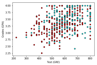
When we plot the data, we get the following graphs, which show that unfortunately, the data is not as nicely separable as we'd hope:
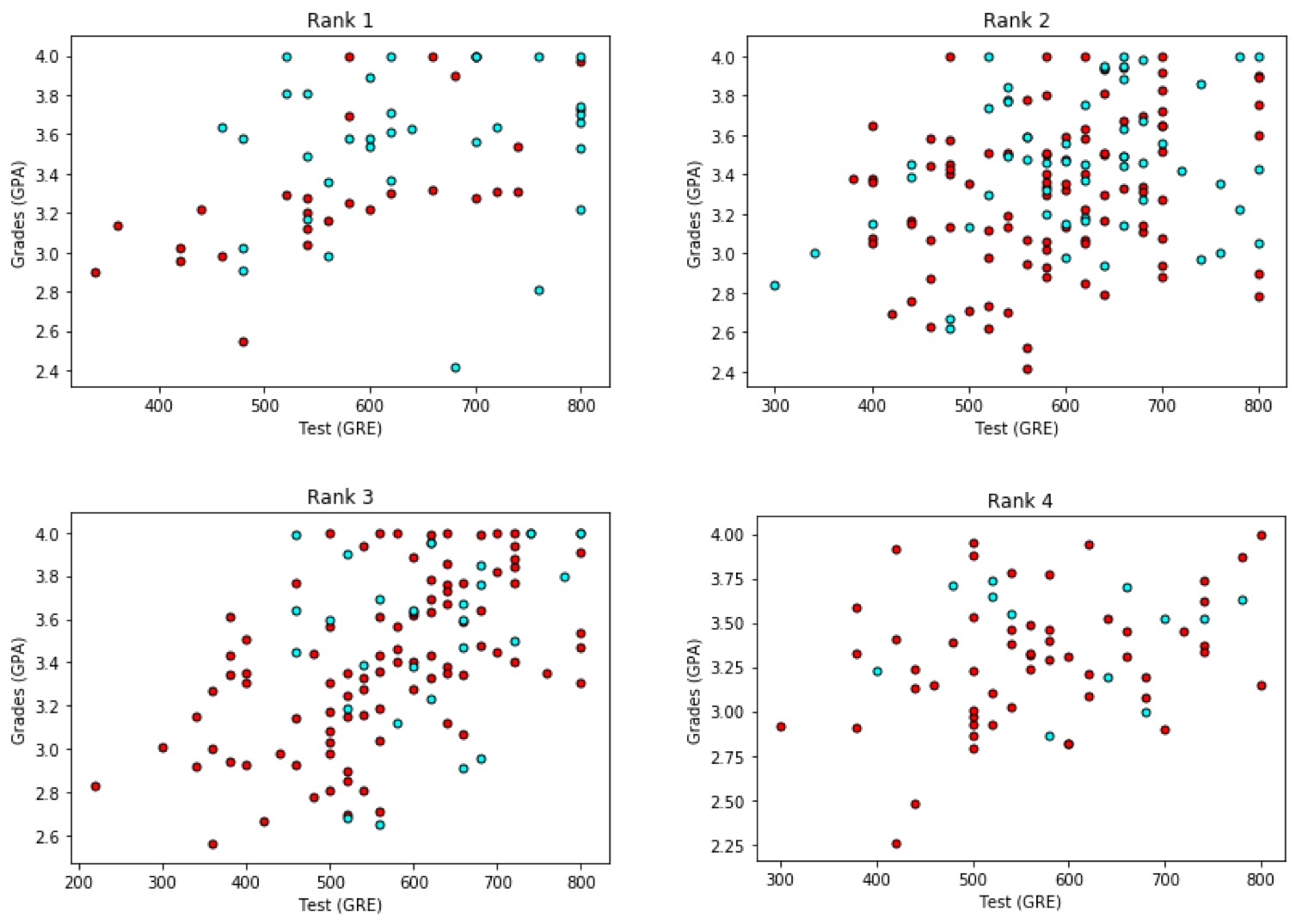
So one thing we can do is make one graph for each of the 4 ranks. In that case, we get this:
Pre-processing the data
Ok, there's a bit more hope here. It seems like the better grades and test scores the student has, the more likely they are to be accepted. And the rank has something to do with it. So what we'll do is, we'll one-hot encode the rank, and our 6 input variables will be:
- Test (GPA)
- Grades (GRE)
- Rank 1
- Rank 2
- Rank 3
- Rank 4.
The last 4 inputs will be binary variables that have a value of 1 if the student has that rank, or 0 otherwise.
So, first things first, let's notice that the test scores have a range of 800, while the grades have a range of 4. This is a huge discrepancy, and it will affect our training. Normally, the best thing to do is to normalize the scores so they are between 0 and 1. We can do this as follows:
 data["gre"] = data["gre"]/800
 data["gpa"] = data["gpa"]/4.0
Now, we split our data input into X, and the labels y , and one-hot encode the output, so it appears as two classes (accepted and not accepted).
 X = np.array(data)[:,1:]
 y = keras.utils.to_categorical(np.array(data["admit"]))
Building the model architecture
And finally, we define the model architecture. We can use different architectures, but here's an example:
model = Sequential()
model.add(Dense(128, input_dim=6))
model.add(Activation('sigmoid'))
model.add(Dense(32))
model.add(Activation('sigmoid'))
model.add(Dense(2))
model.add(Activation('sigmoid'))
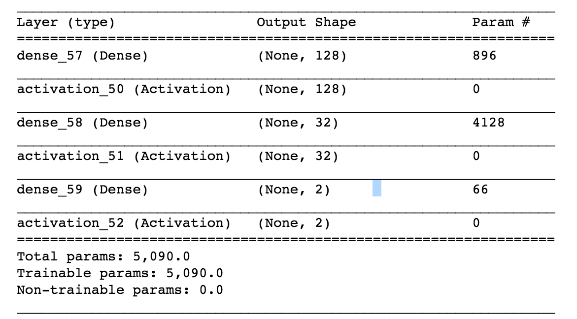
model.compile(loss = 'categorical_crossentropy', optimizer='adam', metrics=['accuracy'])
model.summary()The error function is given by categorical_crossentropy, which is the one we've been using, but there are other options. There are several optimizers which you can choose from in order to improve your training. Here we use adam, but there are others that are useful, such as rmsprop. These use a variety of techniques that we'll outline in upcoming pages in this lesson.
The model summary will tell us the following:
Training the model
Now, we train the model, with 1000 epochs. Don't worry about the batch_size, we'll learn about it soon.
model.fit(X_train, y_train, epochs=1000, batch_size=100, verbose=0)Evaluating the model
And finally, we can evaluate our model.
score = model.evaluate(X_train, y_train)Results may vary, but you should get somewhere over 70% accuracy.
And there you go, you've trained your first neural network to analyze a dataset. Now, in the following pages, you'll learn many techniques to improve the training process.